Interactive simulations & visualizations
Visualizing the beauty in physics and mathematics
Project maintained by zhendrikse Hosted on GitHub Pages — Theme by mattgraham
Somehow it’s okay for people to chuckle about not being good at math. Yet, if I said “I never learned to read,” they’d say I was an illiterate dolt. — Neil deGrasse Tyson
Mathematics
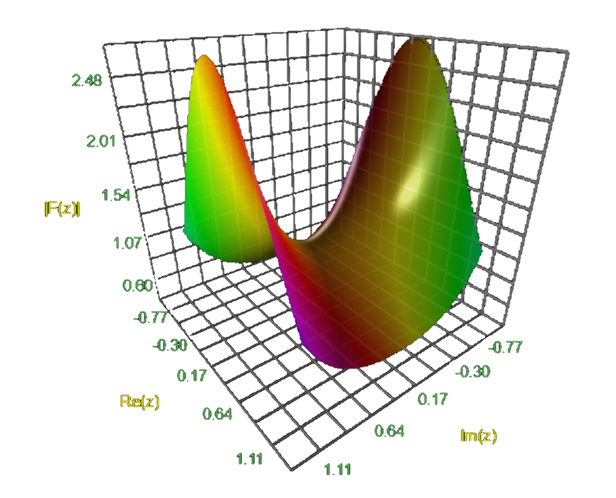
Plots for $f(x, y) \rightarrow \mathbb{R}$
The application below lets one render functions in two real variables $x$ and $y$. The color-coding below is associated with the height of the object and is added purely for aesthetical purposes.
Scalar fields $f(x, y, z) \rightarrow \mathbb{R}$ and vector fields $f(x, y, z) \rightarrow \mathbb{R}^3$
A field is an algebraic structure that is defined as a non-empty collection with two (binary) operations: addition, $a+b$, and multiplication, $a\cdot b$.
These operations are accurately defined by the conditions they must suffice, but roughly speaking they should behave similarly as we know them already from the rational numbers $\mathbb{Q}$ and real numbers $\mathbb{R}$.
The applications below render two such fields, that are abundant in physics, namely scalar fields and vector fields. The former assigns a value (scalar) to every point in space (e.g. the temperature in a room), the latter a vector (e.g. the force and direction of the wind).
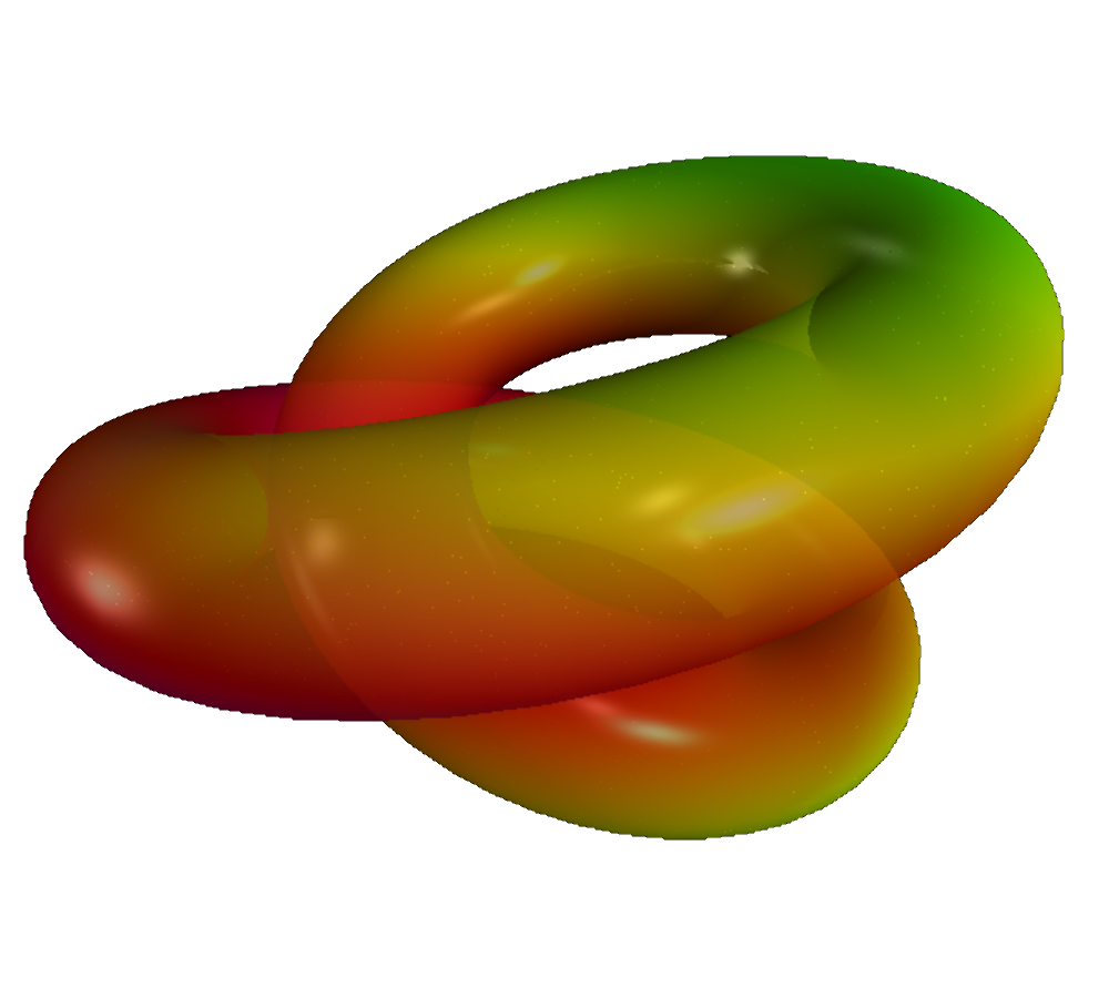
Differential geometry
Games
“If you are curious, you'll find the puzzles around you. If you are determined, you will solve them.” — Erno Rubik.
Mandelbrot & Julia sets
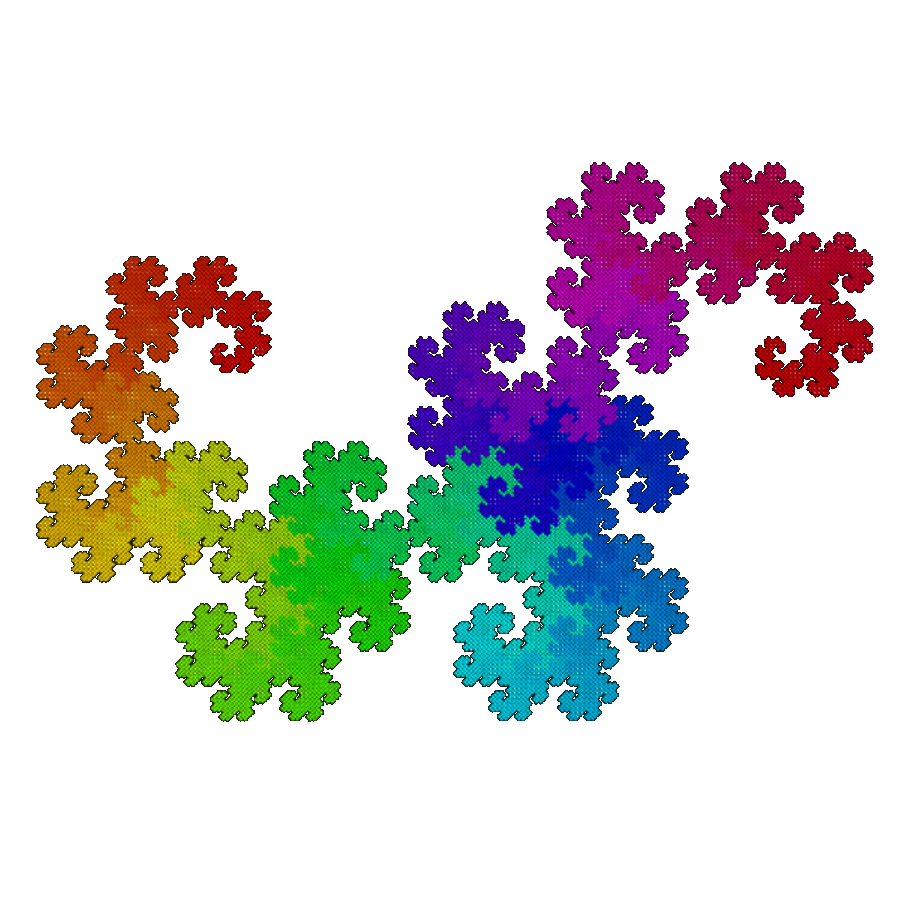
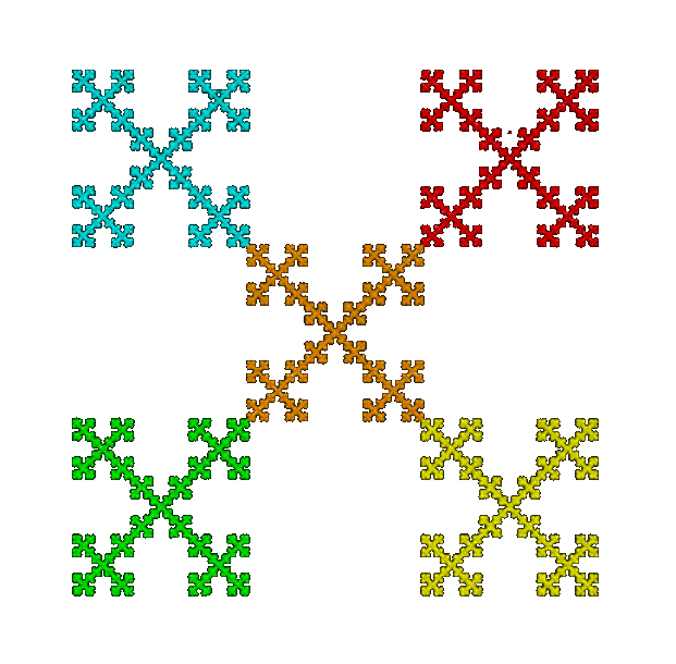
Fractals
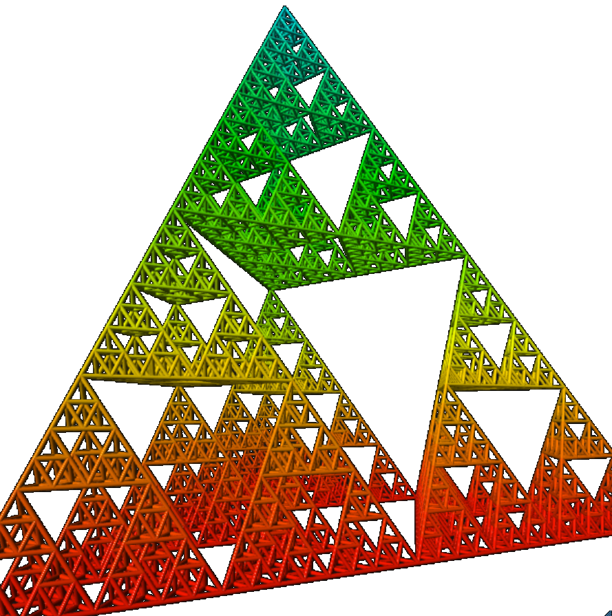
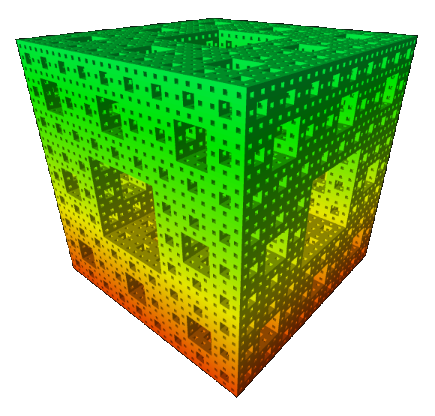
Sierpiński's pyramid & Menger's sponge
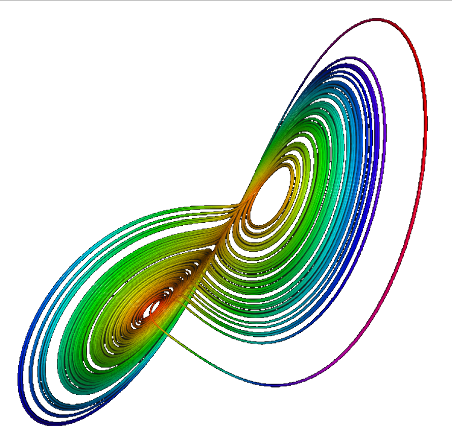
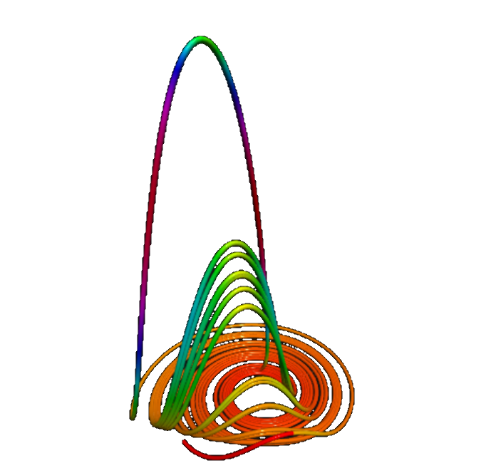
Lorenz & Rössler attractors
Fractal terrains
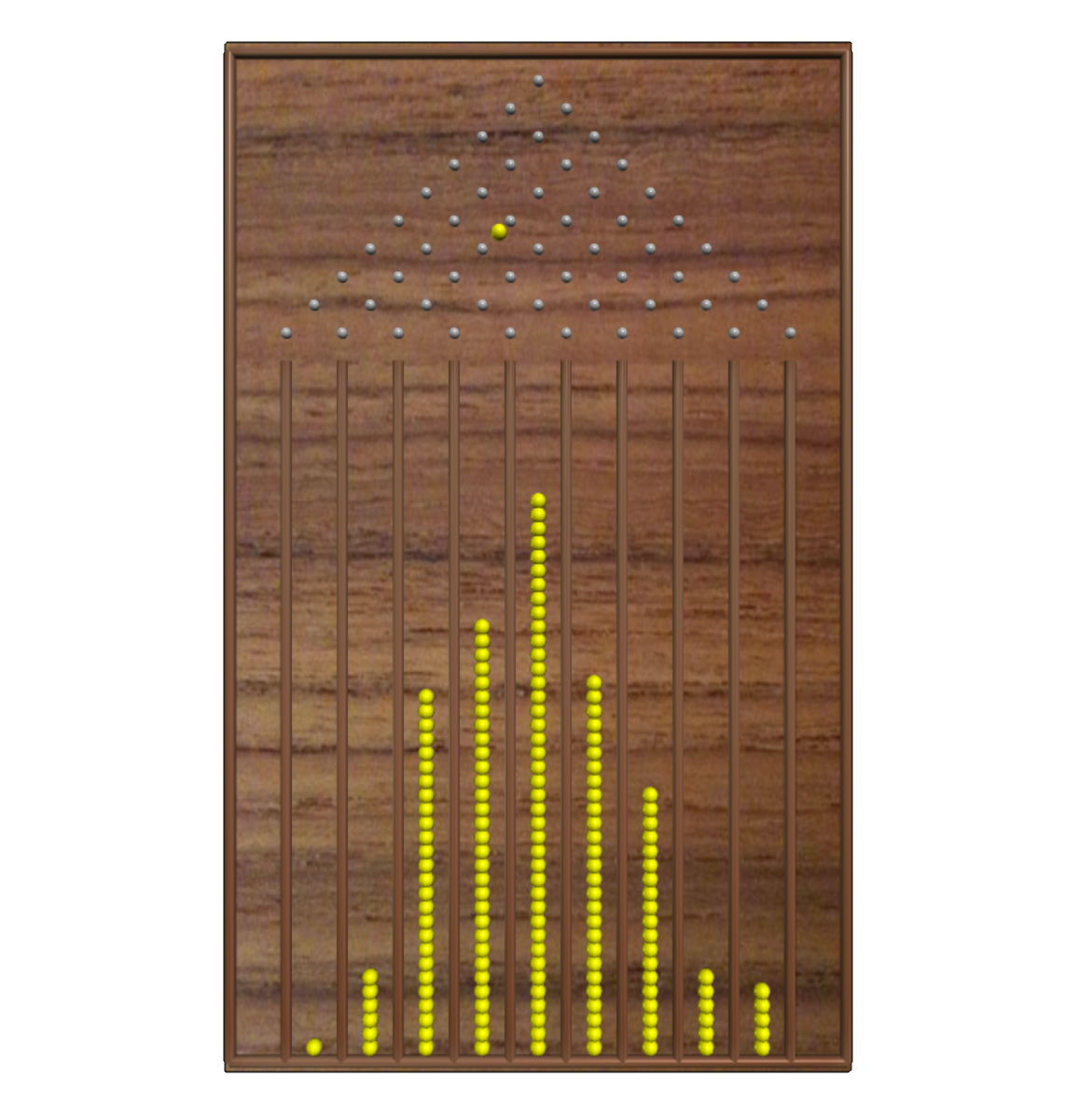
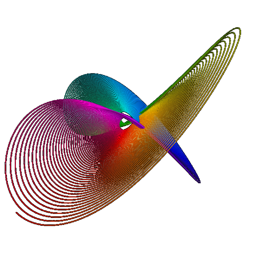
Dalton board and harmonograph
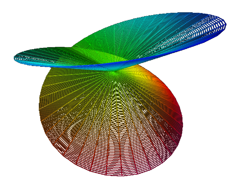
Spherical harmonics
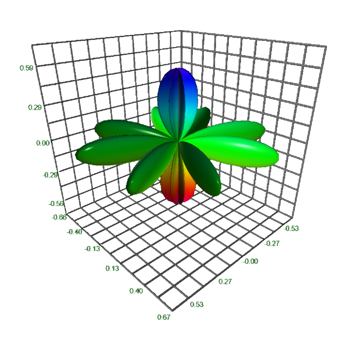
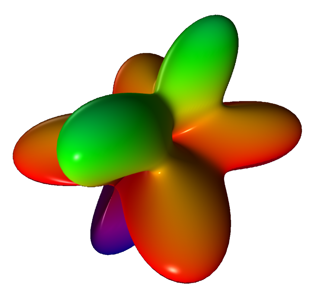
⇓ Python code snippet for plotting spherical harmonics ⇑
The spherical harmonic function is given by $$\begin{cases} \rho & = 4 \cos^2(2\theta)\sin^2(\phi) \\ \theta & = [0, 2\pi] \\ \phi & = [0, \pi] \end{cases}$$ This can then easily be translated to the graphing software, that can also be seen in the mathematics section on this page:def sphere_harmonic():
theta = np.linspace(-1.1 * pi, pi, 100)
phi = np.linspace(0, pi, 100)
U, V = np.meshgrid(theta, phi)
R1 = np.cos(U.multiply(2)).multiply(np.cos(U.multiply(2)))
R2 = np.sin(V).multiply(np.sin(V))
R = R1.multiply(R2).multiply(4)
X = np.sin(U).multiply(np.cos(V)).multiply(R)
Y = np.sin(U).multiply(np.sin(V)).multiply(R)
Z = np.cos(U).multiply(R)
return X, Y, Z, None, None
Numerical methods
References
Computational Physics
- Computational Physics, a freely available online book!
Mathematics
- Geometry, Surfaces, Curves, Polyhedra on Paul Bourke's website.
- Parametric surfaces gallery, a slides presentation with live Three.js-based surfaces
- Manim, an animation engine for explanatory math videos.
- Sage, an open source MatLab on GitHub. Here are some 3D-plot examples.
Share on:
