Interactive simulations & visualizations
Visualizing the beauty in physics and mathematics
Project maintained by zhendrikse Hosted on GitHub Pages — Theme by mattgraham
3D scalar fields
What are you looking at?
This visualization shows how temperature spreads through space.
Each small sphere represents a point in space where we measure the temperature. The color of the sphere tells you how hot it is:
- red / bright colors → hot
- blue / darker colors → cold
Together, all these spheres form a scalar field: a function that assigns one number (temperature) to every point in space.
🔧 This scalar_plot.js is based on Three.js
👉 A VPython version is also available as scalar_plot.py.
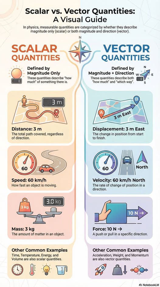
Scalar vis-à-vis vector quantities
The idea of a scalar field
A scalar field is simply a function like
\[T(x, y, z)\]that gives a single value at each position.
Examples of scalar fields:
- temperature in a room
- pressure in the atmosphere
- electric potential
Here, the scalar field represents temperature in 3D space.
Starting situation: a hot spot
At the beginning, the temperature is highest near the center and decreases smoothly outward:
\[T(\mathbf{r}) = e^{-\alpha \lVert \mathbf{r} \rVert^2}\]This describes a localized heat source:
- hottest at the center
- cooler further away
- symmetric in all directions
You can think of this as a small hot object placed in cold space.
What happens over time? (Heat diffusion)
As time passes, heat spreads out due to diffusion.
Mathematically, this is described by the heat equation:
\[\frac{\partial T}{\partial t} = \kappa \nabla^2 T\]You don’t need to solve this equation to understand what happens:
- heat flows from hot regions to cold regions
- sharp peaks smooth out
- the temperature distribution becomes wider and flatter
In the animation, this means:
- colors fade at the center
- warmth spreads outward
- no heat is created or destroyed, it only redistributes
How to read the visualization
- Position of a sphere → where in space we measure temperature
- Color of a sphere → temperature at that position
- Time → how long heat has been spreading
The coordinate axes are only there to help you understand distances and directions.
Why this is useful
This kind of visualization helps you:
- understand abstract functions in 3D
- see what a partial differential equation does, not just how it’s written
- connect mathematics to physical intuition
Instead of thinking in formulas, you can see the heat flow.
Scalar Field Visualization – 🔥 Heat Diffusion 🔥
This visualization shows a three-dimensional scalar field representing a temperature distribution in space.
Each small sphere corresponds to a sample point in ℝ³, where the scalar value is given by a temperature function
\[T(\mathbf{r}, t)\]evaluated at that position. The color of each sphere encodes the local temperature, with warmer colors indicating higher values.
Initial Temperature Distribution
At an initial time, the temperature is modeled as a radially symmetric Gaussian field:
\[T(\mathbf{r}) = e^{-\alpha \lVert \mathbf{r} \rVert^2},\]where:
- $\mathbf{r} = (x, y, z)$ is the position vector,
- $\alpha > 0$ controls how rapidly the temperature decays with distance.
This represents a localized heat concentration centered at the origin.
Time-Dependent Heat Diffusion
The time evolution of the temperature follows the fundamental solution of the three-dimensional heat equation:
\[\frac{\partial T}{\partial t} = \kappa \nabla^2 T,\]with thermal diffusivity $\kappa$.
The analytical solution for a point-like heat source is:
\[T(\mathbf{r}, t)= \exp\left( -\frac{\lVert( \mathbf{r} \rVert^2}{4\kappa t} \right), \qquad t > 0.\]As time increases:
- the peak temperature decreases,
- heat spreads outward,
- the distribution becomes broader and flatter.
Visualization Details
- The scalar field is sampled on a uniform 3D grid.
- Each grid point is rendered as a semi-transparent sphere.
- Color encodes temperature magnitude.
- The coordinate axes are shown for spatial reference but do not affect the field itself.
This visualization provides an intuitive, geometric view of scalar fields and diffusive processes in three dimensions.
Share on: