Interactive three-dimensional simulations & visualizations
Visualizing the beauty in physics and mathematics
Project maintained by zhendrikse Hosted on GitHub Pages — Theme by mattgraham
Vector fields & implied flow
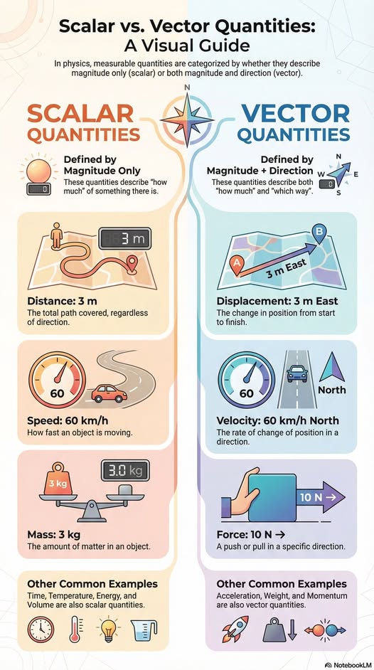
Scalar vis-à-vis vector quantities
What do the colors show?
Given a vector field $F = (u, v, w)$, the divergence is defined by
\[\nabla \cdot \mathbf{F} = \frac{\partial u}{\partial x} + \frac{\partial v}{\partial y} + \frac{\partial w}{\partial z}\]Interpretation:
🔴 positive → source
🔵 negative → sink
⚪ zero → incompressible
The curl is defined by
\[\nabla \times \mathbf{F}\]For the color we use the magnitude of the curl: \(||\nabla \times \mathbf{F}||\)
Interpretation:
- local magnitude of rotation behavior
- vortex-structures become directly visible
The vector field is sampled on a lattice, so we apply central differences.
For the divergence this leads to
∂u/∂x ≈ (u(x+dx) − u(x−dx)) / (2dx)
∂u/∂y ≈ (u(y+dy) − u(y−dy)) / (2dy)
∂u/∂z ≈ (u(z+dz) − u(z−dz)) / (2dz)
and the curl
curl_x = ∂w/∂y − ∂v/∂z
curl_y = ∂u/∂z − ∂w/∂x
curl_z = ∂v/∂x − ∂u/∂y
Summarizing:
| Property | Channel |
|---|---|
| Direction | Arrow orientation |
| Strength | length |
| Divergence | color |
| Rotation | curl-color |
| Time | animation |
Possible extensions
In the future, the following may be added:
🧭 streamlines / pathlines
🧠 Helmholtz-decompositie
📊 interactieve colorbar
⚡ GPU finite differences (shader)
🌀 curl-vectors as opposed to magnitude
Share on: