🔦 Fraunhofer diffraction

About

🎯 Proving the wave-like nature of light using physical optics visualization
🎯 Demonstration of rendering a scalar grid/intensity field
🧠 Simulation inspired by this video by Jordan Huang
🐍 A VPython demo is available as well, see circular_aperture.py
👉 Related to fourier transformation

Below you’ll find a diffraction pattern of an aperture (circular or rectangular) far away from a screen, also known as Fraunhofer diffraction. The intensity is calculated as the square of the amplitude of the electric field.

Live demo

Instructions given in the video

Since the original video is in Chinese, you can find a copy of the original set of instructions that accompany the video below.

$r = \sqrt{(x-X)^2 + (y-Y)^2 +z^2} = \sqrt{x^2+y^2+z^2-2xX-2yY+X^2+Y^2}$

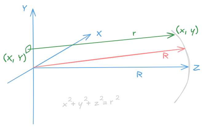
Extracting $R$ results in

$r=R\sqrt{1-\dfrac{2xY+2yY}{R^2}+\dfrac{X^2+Y^2}{R^2}}$

For a small aperture we have $X^2+Y^2 \ll R^2$, so we can write

$r \approx R\sqrt{1-\dfrac{2xY+2yY}{R^2}} \approx R\left(1-\dfrac{2xY+2yY}{R^2}\right)$

I. Original homework assignment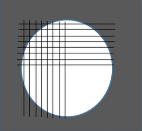

This homework is to find the diffraction pattern of a circular aperture far from the screen. Assume there is a circular aperture of diameter $d=100 \mu m$ and there is a spherical screen at $R=1m$ away. The light source is of wavelength $\lambda=500nm$. To obtain the diffraction pattern, you can assume there are many point light sources at the lattice points, sitting at the cross points of the $N=100$ vertical lines and $N=100$ horizontal lines, each separated by $s=d/N=1\mu m$ apart. If the lattice point’s position is within the circular aperture, then it is allowed to radiate light. Then on the screen you add all the electric field contributions from the light sources of the grid points, and you will be able to obtain the diffraction intensity pattern by squaring the electric field (the detailed derivation is listed in the next page).

In addition to generating the intensity plot of the diffraction pattern, also find and print the radius of the first dark ring and check whether the Rayleigh criterion $\theta=1.22\lambda / d$ is satisfied. Also notice that, to calculate intensity is to do the square of the amplitude. However, the ‘real’ diffraction pattern is really faint to be observed on the computer screen. Therefore, we also do a ‘false’ intensity image of the diffraction pattern by taking the absolute value of the amplitude as the intensity. Of course, when you want to calculate the radius of the first dark ring, you should use the ‘real’ intensity image.

II. Theoretical background

The amplitude of the electric field at position $(x, y)$ on the screen gets its contribution from all point sources sitting inside the aperture

$$E(x, y) =\int\int_{\text{aperture}} \dfrac{1}{r}\sin(\omega t - kr)dXdY$$

Next, we substitute the expression for $r$ found in the previous section to obtain

$$E(x, y) \approx \int\int\dfrac{1}{R\left(1 - \dfrac{xX + yY}{R^2}\right)}\sin\left(\omega t - kR\left(1 -\dfrac{xX + yY}{R^2}\right)\right)dXdY$$

Now let $\theta_x=x/R, \theta_y=y/R, k_x=k\theta_x, k_y=k\theta_y$, then

$$E(\theta_x, \theta_y) \approx \int\int \frac{1}{R}\sin(\omega t -kR +k_x X + k_y Y)dXdY$$

Applying some basic trigonometry we get

$$\begin{split} E(\theta_x, \theta_y) \approx \int\int \frac{1}{R}\sin(\omega t -kR)\cos(k_x X + k_y Y)dXdY + \\ \int\int \frac{1}{R}\cos(\omega t -kR)\sin(k_x X + k_y Y)dXdY \end{split}$$

which is equivalent to

$$\begin{split} E(\theta_x, \theta_y) \approx \sin(\omega t -kR)\int\int \frac{1}{R}\cos(k_x X + k_y Y)dXdY + \\ \cos(\omega t -kR)\int\int \frac{1}{R}\sin(k_x X + k_y Y)dXdY \end{split}$$

As we have

$$\int\int \frac{1}{R}\sin(k_x X + k_y Y)dXdY=0$$

due to the symmetry of the integration on the “circular” aperture (between quotes, since we have approximated it by a square area in our code), we get

$$E(\theta_x, \theta_y) \approx \sin(\omega t -kR)\int\int \frac{1}{R}\cos(k_x X + k_y Y)dXdY = A \cdot \sin(\omega t -kR)$$

where

$$A = \int\int_\text{aperture} \frac{1}{R}\cos(k_x X + k_y Y)dXdY$$

is the amplitude of the electric field on the spherical screen, which is the one you should calculate by summation over all the grid points on the aperture.

This formula for the amplitude $A$ can then directly be translated into code:

class ElectricField {
// ...

_computeElectricField(aperture, lambdaInNanoMeter) {
    const k = 2 * Math.PI / (lambdaInNanoMeter * 1e-9);
    for (let i = 0; i < this._N; i++)
        for (let j = 0; j < this._N; j++)
            this._field[i][j] = aperture.sumRaysAt(i, j, k) / R;
}
}

class Aperture {
// ...

sumRaysAt(i, j, k) {
    let field = 0;
    const kx = k * this._kX[i][j];
    const ky = k * this._kY[i][j];

    for (const [m, n] of this._aperture)
        field += Math.cos(kx * this._X[m][n] + ky * this._Y[m][n]) * this._dx_dy;

    return field;
}
}