⚡ Static electric fields

Field of a dipole

About

🎯 Visualization of electric dipole field
🧠 Inspired by 7_Dipole.py
🐍 A VPython demo is available as well, see dipole_field.py
👉 Electric dipole field formula:

$$\overrightarrow{E} ( \overrightarrow{r} ) = -\frac {1} {4\pi\epsilon_0} \nabla \bigg( \frac{\overrightarrow{r} \cdot \overrightarrow{p}} {r^3} \bigg),\quad \overrightarrow{p} = q(\overrightarrow{r}_+) -q(\overrightarrow{r}_-)$$

Live experiment

Field of a solenoid ➿

About

🎯 Electric field around a solenoid
🧠 Inspired by 25-4.Bsolenoid
👉 Field vectors are rendered on a logarithmic scale
🐍 A VPython demo is available as well, see solenoid.py

Live experiment

💪 Potential fields

🎯 Electric field of a non-ideal capacitor
🧠 Inspired by this video by Jordan Huang
🐍 A VPython demo is available as well, see non_ideal_capacitor.py

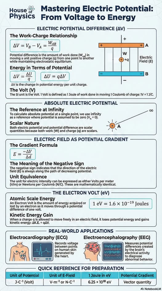
Electric potential difference $\Delta V$

Theoretical background

The capacity for a capacitor consisting of two parallel plates is given by $C = \epsilon_0A/d$, where $A$ is the surface area and $d$ the distance between the plates, and $\epsilon_0$ the permittivity of the spacer material.

Since $d \ll A$, we expect the fields to be approximately constant with $\rho$ until we get close to the edge of the plates. Therefore, we assume $\partial V/\partial\rho$ is negligible and can be taken to be zero. As the surrounding area does not contain any additional charges, we can consider this to be a so-called source-free region, and Laplace’s Equation applies:

$$\nabla^2V=0$$

A reasonable question to ask at this point would be, what about the potential field close to the edge of the plates, or, for that matter, beyond the plates? The field in this region is referred to as a fringing field. For the fringing field, $\partial V/\partial \rho$ is no longer negligible and must be taken into account.

In addition, it is necessary to modify the boundary conditions to account for the outside surfaces of the plates (that is, the sides of the plates that face away from the dielectric) and to account for the effect of the boundary between the spacer material and free space. These issues make the problem much more difficult. When an accurate calculation of a fringing field is necessary, it is common to resort to a numerical solution of Laplace’s Equation. Fortunately, accurate calculation of fringing fields is usually not required in practical engineering applications. — www.circuitbread.com

When we assume the plates to lie in the $xy$-plane, the fields will be symmetric along the $z$-direction, hence $\partial/V\partial z$ will be zero.

This simplifies our Laplace equation to

$$\dfrac{\partial^2V}{\partial x^2} + \dfrac{\partial^2V}{\partial y^2} = 0$$

Once we know the potential $V$, we can also calculate the electric field:

$$\vec{E} = -\nabla\cdot V = -\left( \dfrac{\partial}{\partial x}\hat{x} + \dfrac{\partial}{\partial y}\hat{y} + \dfrac{\partial}{\partial z}\hat{z} \right)V$$

So our task is to numerically solve the second order differential equation for the potential $V$:

• $V(x + h, y) \approx V(x, y) + h\dfrac{\partial V}{\partial x} + \dfrac{h^2}{2}\dfrac{\partial^2 V}{\partial x^2}$

• $V(x, y + h) \approx V(x, y) + h\dfrac{\partial V}{\partial y} + \dfrac{h^2}{2}\dfrac{\partial^2 V}{\partial y^2}$

• $V(x - h, y) \approx V(x, y) - h\dfrac{\partial V}{\partial x} + \dfrac{h^2}{2}\dfrac{\partial^2 V}{\partial x^2}$

• $V(x, y - h) \approx V(x, y) - h\dfrac{\partial V}{\partial y} + \dfrac{h^2}{2}\dfrac{\partial^2 V}{\partial y^2}$

$$V(x, y) = \dfrac{1}{4} \bigg( V(x + h, y) + V(x, y+ h) + V(x - h, y) + V(x, y - h) \bigg)$$

This translates to the following JavaScript code:

export class LaplaceOperator {
    static at(field, i, j) {
        return (
            field.valueAt(i + 1, j) +
            field.valueAt(i - 1, j) +
            field.valueAt(i, j + 1) +
            field.valueAt(i, j - 1) -
            4 * field.valueAt(i, j)
        );
    }
}

The electric field

$$\overrightarrow{E} =-\overrightarrow{\nabla} V$$

is then calculated in a similar way:

$$E_x=-\frac{V_{i+1,j}-V_{i-1,j}}{2h}, \qquad E_y=-\frac{V_{i,j+1}-V_{i,j-1}}{2h}$$

Infographics

This visual originates from House of Physics.

This visual originates from House of Physics.

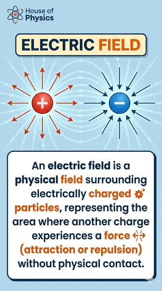
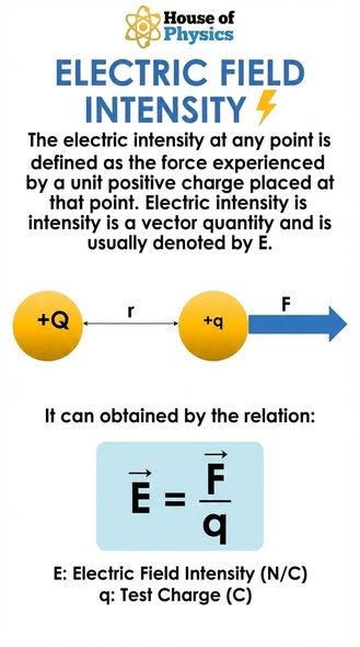
Capacitor fields

This excellent visual guide originates from House of Physics.