📐 Differential geometry

About

🎯 Illustration of visualizing parametric geometries with Helion

\phi(u, v): \mathbb{R}^2 \rightarrow \mathbb{R}^3

Parametric surfaces

Calculation of classic shape invariants

The following shape invariants are (numerically) calculated and can subsequently be visualized:

Height
Gaussian curvature
Mean curvature
Principal curvature 1
Principal curvature 2
Shape Index
Curvedness

Shape index and curvedness are often encountered together, because roughly speaking the shape index tells us something about the shape itself, and the curvedness tells us something about the magnitude of the curvature.

S = \frac{2}{\pi} \arctan\left(\frac{k_1+k_2}{k_1-k_2}\right)

C = \sqrt{\frac{k_1^2+k_2^2}{2}}

Numeric calculation of shape invariants

We use central differences of second order for all derivatives as these derivatives are

translation-invariant
no preferred direction
stable for curvature calculations

This is essential for:

correct signs of $k_1$ and $k_2$
correct ratio between both $k_1$ and $k_2$

Note that forward differencing is asymmetric and leads to an error in the curvature calculation.

For central differences we use:

X_{uu} = \frac{X(u+e)-2X(u)+X(u-e)}{e^2}

X_{uv} = \frac{ X(u+e,v+e)-X(u+e,v-e)-X(u-e,v+e)+X(u-e,v-e)}{4e^2}

Comparison with analytic Gaussian curvature of a torus

For a torus with major radius $R$ and minor radius $r$ we have the following parametrization:

X(u,v) = \begin{pmatrix} (R + r\cos v)\cos u \\ (R + r\cos v)\sin u \\ r\sin v \end{pmatrix}

⭐ The Gaussian curvature is given by:

K(v) = \frac{\cos v}{r (R + r \cos v)}

👉 Note that this curvature

is independent of u,
is zero at $v = \pm\frac{\pi}{2}$ ,
and has a change of sign between the blue ↔ red transition.

For the coloring this means that:

🔴 Outside where $\theta = 0 \rightarrow \cos\theta = 1 \rightarrow K > 0$ : elliptic, e.g. red
🔵 Inside where $\theta = \pi \rightarrow \cos\theta = -1 \rightarrow K < 0$ : hyperbolic, e.g. blue
⚪ Side lines where $\theta = \pm \dfrac{\pi}{2} \rightarrow K = 0$ : parabolic

For the principal curvature $k_1$ we observe that

🔴 Outside strongly positive (red)
🔵 Inside: strongly negative (blue)

and for $k_2$ that it has the same sign everywhere with varying intensity.

🧠 Summarizing, a torus has

both positive and negative Gaussian curvature
two closed K = 0-contours (the so-called “equatorial” circles)
no contours where the mean curvature $H = 0$

Helion implementation details

Color mapping

There are three kinds of scalar fields. Depending on the scalar field, the program automatically changes to the preferred color mapping of the scalar field (shape invariant) of choice.

1. Sign-sensitive (positief / negatief)

Gaussian curvature ( $K$ )
Mean curvature ( $H$ )
Shape index (partly)

This implies a divergent color mapping with zero as neutral is preferred.

2. Magnitude-only (alleen grootte)

Curvedness
$|H|$
$|K|$
velocity magnitude etc.

This implies a preference for a monotonic colormap without “zero-centering”.

3. Bounded semantic range

Shape index ∈ [-1, 1]

Here a symmetric and perceptually uniform mapping is preferred.

Design

=> ParametricSurface (math surface def, e.g. torus)
          ↓
        Feeds
          ↓
=> DifferentialGeometry
          ↓
      results in
          ↓
=> GaussianCurvatureField (scalar field)
          ↓
       value to
          ↓
=> NormalizedScalarField
          ↓
      value to
          ↓
=> ColorMapper (maps [0, 1] -> color)
          ↓
       used by
          ↓
=> PlaneSurfaceView (view on math surface)

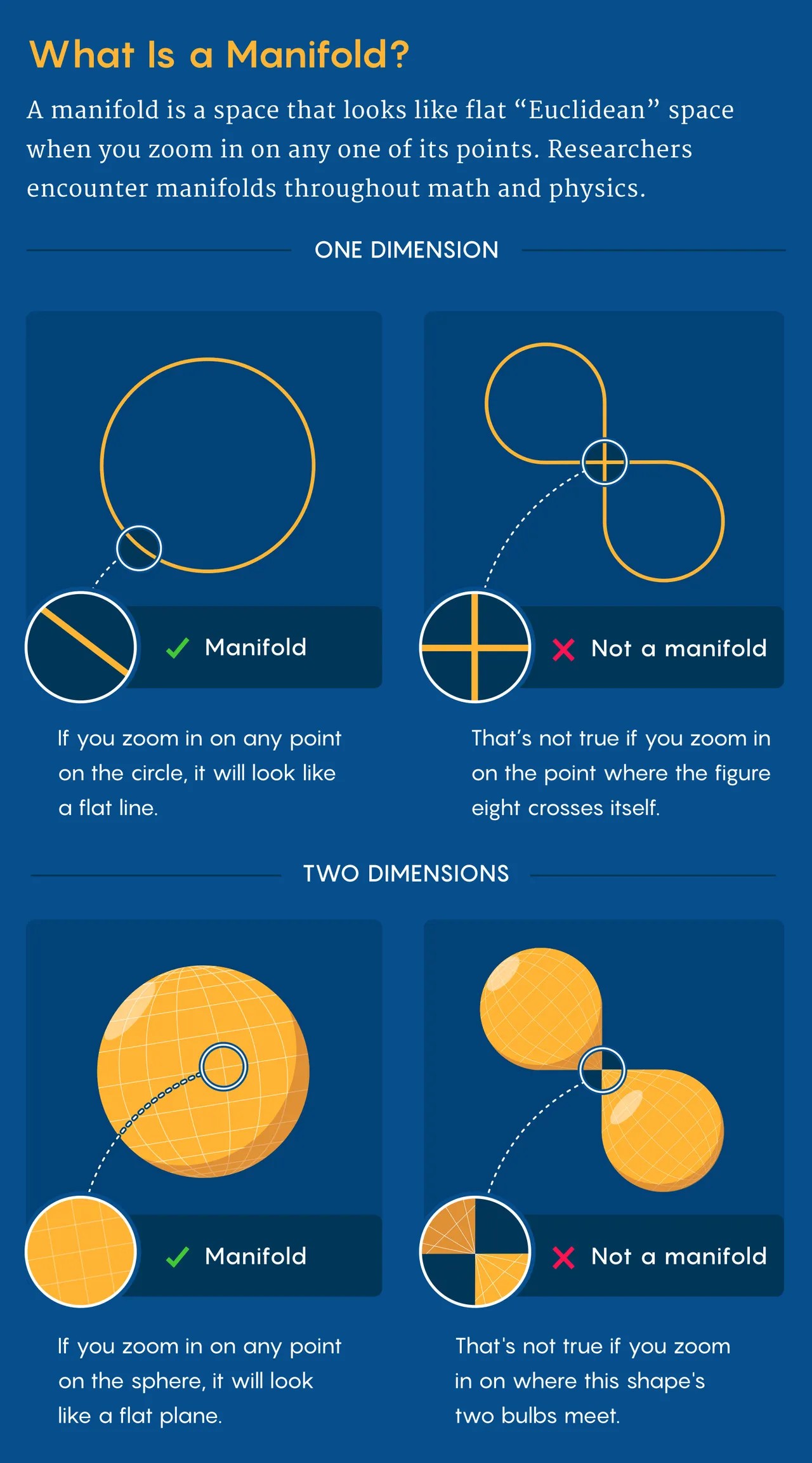
On manifolds

From: Behold the Manifold, the Concept that Changed How Mathematicians View Space:

The term “manifold” comes from Riemann’s Mannigfaltigkeit, which is German for “variety” or “multiplicity.”

A manifold is a space that looks Euclidean when you zoom in on any one of its points. For instance, a circle is a one-dimensional manifold. Zoom in anywhere on it, and it will look like a straight line. An ant living on the circle will never know that it’s actually round. But zoom in on a figure eight, right at the point where it crosses itself, and it will never look like a straight line. The ant will realize at that intersection point that it’s not in a Euclidean space. A figure eight is therefore not a manifold.

Similarly, in two dimensions, the surface of the Earth is a manifold; zoom in far enough anywhere on it, and it’ll look like a flat 2D plane. But the surface of a double cone — a shape consisting of two cones connected at their tips — is not a manifold.

Introduction to manifolds — From Behold the Manifold, the Concept that Changed How Mathematicians View Space..