Interactive three-dimensional simulations & visualizations

Visualizing the beauty in physics and mathematics

---

Project maintained by zhendrikse Hosted on GitHub Pages — Theme by mattgraham

Zeger's home / Science home / Relativity /

A comet moving in Schwarzschild space-time

Visualization explained

The application is best described in Ryston's article itself:

• Motion of marbles rolling on bend surface affected by actual gravity and friction — naturally, when we use a simulation, we don’t have to deal with non-ideal conditions of real world experiments. Point-like particles can be made to move strictly in the surface without friction and without any force acting on them, their motion being affected purely by the curvature of the surface. To support the idea that the motion is restricted to the surface, it is beneficial to be able to flip the whole embedding diagram upside down, a feature that is easily achieved with a simulation but hardly with a real aperture.
• Emphasis on the two-dimensional motion — as we mentioned above, the only physically relevant part of the motion is in the horizontal plane (𝑟, 𝜑) or (𝑥, 𝑦), if you will. With a rotatable simulation, we can take advantage of a view from the top (looking in the direction of the 𝑧 axis). In this view, we see purely the effect of spatial curvature on the motion. Taking advantage of the simulation further, we can add a second particle which will follow the motion of the first particle but only in the horizontal plane. This way we can point out the difference in the two motions and how they are related. It would be most interesting to see such a setup with the marbles, but one can imagine achieving that could be extremely difficult.
• Purely spatial curvature — needless to say, this is the one conceptual obstacle that we cannot get rid of when using this type of embedding diagram, and we need to keep it in mind. However, what we can do is add another particle moving in the horizontal plane whose motion will start with the same initial conditions as the particle on the curved surface but which moves according to the complete set of equations of motion for the equatorial plane of Schwarzschild spacetime. This mainly means adding the time component, which substantially changes the motion. This feature allows the user to, at least qualitatively, compare the “real” motion with the one due to space curvature. A practical note: In order to clearly see the curvature of the embedding diagram and its effect on the motion, we usually visualize a region of space that is very close to the Schwarzschild horizon, which means that the real-motion particle almost immediately falls inside the central object. Therefore, this feature serves only as a rough comparison of the two motions.
• Dynamical changes of the curvature — lastly, let us mention a nice feature that is again possible only using a computer simulation. By changing the central mass parameter 𝑀 of the curvature (see equations above), we can change the curvature dynamically, even during a particles motion. While this hardly corresponds to a real world situation (the central gravitating body would have to lose mass while remaining spherically symmetric and without rotation), it is an interesting feature enabling us to compare trajectories for different curvatures. In other words, we can show the perhaps intuitive, fact that larger mass curves space around itself more, resulting in stronger curving of the trajectories

Theoretical background

The Schwarzschild metric describes a gravitational field of a non-rotating spherical mass (and without electric charge), see Wikipedia:

$\begin{equation}ds^2=cd\tau^2=\left(1-\dfrac{r_s}{r}\right)c^2dt^2-\left(1-\dfrac{r_s}{r}\right)^{-1}dr^2-r^2d\Omega^2\end{equation}$

where

$\begin{equation}d\Omega^2=\left(d\theta^2 + \sin^2\theta d\phi^2\right) \text{, } r_s=\dfrac{2GM}{c^2}\end{equation}$

and $G$ is Newton’s gravitational constant, $c$ the speed of light and $M$ is the mass of the non-rotating spherical object.

When we assume the time to be constant ($dt=0$), we get:

$\begin{equation}ds^2 = \dfrac{dr^2}{1 - \dfrac{2GM}{c^2r}} +r^2d\phi^2\end{equation}$

Now, according to Ryston's article:

In order to visualize the curvature in the 𝑟 direction, we embed this surface into the three-dimensional Cartesian space (where 𝑟 and 𝜑 are identical to polar coordinates and the third, vertical Cartesian coordinate 𝑧 is used to visualize the actual curvature – see figure 1 below). As a result, we get an equation for the 𝑧 coordinate as a function of 𝑟:

$z(r)=\sqrt{\dfrac{8GMr}{c^2} - \dfrac{16M^2g^2}{c^4}}$

Of course, this equation 𝑟 and 𝑧 are in meters, which is not very convenient for visualizing large regions of space. For this reason, geometricized units where 𝑐 = 𝐺 = 1 are often used. Then we get the simpler form:

$z(r) = \sqrt{8Mr - 16M^2}$.

Figure 1:The-exterior t=const equatorial plane of a Schwarzschild Black Hole from Spacetime Embedding Diagrams for Black Holes.

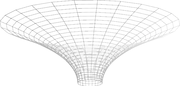
This is the quintessential formula that is used in this visualization:

class SchwarzschildSpaceTime:
    def __init__(self, mass, grid_y_offset=-10):
        self._mass = mass
        # ...
    
    # ...

    def z_as_function_of(self, r):
        return sqrt(8 * self._mass * r - 16 * self._mass * self._mass)